PEYTON MURRAY

I've been playing around with blender again.

Blender, again

I'd been thinking about submitting something for this year's John D. Hunter Excellence in Plotting Contest, but as it turned out I went away for about a week leading up to the final submission date, and didn't have anything prepared by the last day. I struggled for a few hours before the deadline to come up with something worth submitting, but nothing I tried seemed as visually impressive as I originally hoped it would be. Ultimately I just didn't have enough time to submit an entry, because I had made plans to travel with my parents on the final submission day, and I wasn't about to put off going on an awesome trip (Helsinki!) to make figures. But after returning from my trip, I wanted to complete my original goal: use Blender to make a visualization of something related to magnetism.

Back to Blender. Previously I made a post about how you can import scientific data into Paraview, manipulate it, and export the result as a PLY file, which can then be imported into Blender for fancy visualization. That method is, for me, still the easiest way to produce great still images. There are however a few important shortcomings to consider before using this method:

1. Vertex colors just don't work with Eevee, the incredible new render engine introduced in Blender 2.8. This means you're restricted to using the Cycles engine, which is more accurate than Eevee but much, much slower.
2. Animations are almost impossible to make, in part because this method requires a lot of intermediate files (raw data -> VTK -> PLY -> Blender save) which take up a ton of disk space. Since you need a PLY file for each frame of an animation, the amount of storage you need for any sizeable dataset quickly grows beyond a reasonable size.
3. Because the PLY files generated by Paraview export all of the objects in view as a single mesh, they aren't really separate in any real sense in Blender. This means you can't do cool stuff like keyframing the properties of the objects you imported. They aren't really separate objects at all; the imported PLY is just a single object with a single mesh.¹ For these reasons I needed to find another way to visualize my data. Fortunately, pretty much everything that you can do with the Blender GUI can also be done using the powerful python API, which makes reading in data really straightforward.

How are magnetic materials simulated?

I really wanted to make an animation of how a ferromagnet reacts in response to a magnetic field; I've never seen any simulations showing the process (outside of academic papers and talks), and I think it has the potential to be visually appealing while still being understandable for non-scientists. On the microscopic scale, you can think of a magnetic material as being composed of many small bar magnets:

When a magnetic field is applied, these small magnets move and reorient themselves to align with the applied magnetic field. So the idea is to first simulate the motion of these microscopic magnetic moments and then visualize their motion in Blender. To produce the data I'll eventually be reading into Blender, I used the Mumax3 micromagnetics simulation package. In a nutshell, Mumax simulates the behavior of magnetic materials on the nanoscale by dividing up the simulated material into little cubic cells, each with its own magnetic moment. These little magnetic moments then are allowed to interact with each other according to the Landau-Lifshitz-Gilbert equation, which describes how the little magnets move. The simulations shown here show how a thin, planar layer of perpendicularly magnetized material reacts when a magnetic field is applied out-of-plane.

To run a simulation, Mumax needs a configuration file which describes what kind of magnetic material you'd like it to simulate, what shape the materials is, and a number of other important parameters. As part of this configuration file, you can specify a number of options related to data output - what type of data you'd like, how often the magnetization is recorded, and so on. Usually, you would configure Mumax to write the magnetization of every simulation cell to a file every so often - say, every $10^{-12}$ seconds. The resulting files would contain the (x, y, z) locations and (mx, my, mz) spin vectors of the magnetization for each cell. Unfortunately this data isn't very useful to import into Blender because there's doesn't seem to be an easy way to take a Blender object - such as a cone - and align it along a certain vector².

Making a plan

To get around this limitation, I'll make use of Blender's Axis Angle rotation mode, which allows any object to be rotated around an arbitrary axis (given by a vector $\textbf{k}$) by a specified angle $\theta$. This transformation makes use of Rodrigues' rotation formula,

which rotates the original vector $\textbf{v}$ into a new direction $\textbf{v}_{rot}$. Now the process of animating the simulated data in Blender becomes straightforward:

1. Create a cone at each cell location (x, y, z).
2. Set all of the rotation angles of the cones to 0. This orients the cones along the $+\hat{z}$-direction, i.e. $\textbf{v} = (0, 0, 1)$.
3. Read in the magnetization data $\textbf{v}_{rot}$ for the current timestep from the simulation.
4. For each cone, calculate $\theta$ and $\textbf{k}$ from the simulation data. Apply the Axis Angle transformation.
5. Keyframe the rotation of the cones.
6. Move to the next timestep and repeat from step 2.

Now the main problem is finding $\theta$ and $\textbf{k}$, but this isn't actually very hard. By default, the cones start out pointing up: $\textbf{v} = (0, 0, 1)$, and we want to use Blender to rotate $\textbf{v}$ to align with the magnetization data $\textbf{v}_{rot}$. This can always be done by choosing a rotation axis $\textbf{k}$ which lies in in the $xy$-plane. To find a direction of $\textbf{k}$ which works, just take the cross product $\textbf{v} \times \textbf{v}_{rot}$, which always points at right angles to both vectors. What about $\theta$? Well, since the cones start out pointing up, $\theta$ is just the same old polar angle you encounter whenever you use cylindrical coordinates! In summary:

Implementation

I started out by writing Go functions to allow the Mumax simulator to export the location of all the simulation cells. The resulting cellLocs.csv file has the indices and location of each cell:

#ix,iy,iz,x,y,z
0,0,0,5.000000E-10,5.000000E-10,5.000000E-10
1,0,0,1.500000E-09,5.000000E-10,5.000000E-10
2,0,0,2.500000E-09,5.000000E-10,5.000000E-10
3,0,0,3.500000E-09,5.000000E-10,5.000000E-10
4,0,0,4.500000E-09,5.000000E-10,5.000000E-10
⋮

I also wrote Go functions to write a .csv file at every time step of the simulation. The resulting files looked like this:

#time = 7.950000E-09
#ix,iy,iz,kx,ky,kz,angle
0,0,0,7.121113E-01,-7.020666E-01,0.000000E+00,4.882812E-04
1,0,0,7.076833E-01,-7.065297E-01,0.000000E+00,4.882812E-04
2,0,0,7.037417E-01,-7.104561E-01,0.000000E+00,4.882812E-04
3,0,0,7.011437E-01,-7.130199E-01,0.000000E+00,4.882812E-04
4,0,0,6.999333E-01,-7.142082E-01,0.000000E+00,4.882812E-04
5,0,0,7.000152E-01,-7.141279E-01,0.000000E+00,4.882812E-04
⋮

At the top, there's a header showing the current simulation time and the column names. (ix, iy, iz) are the (x, y, z) indices of each simulation cell; (kx, ky, kz) is the rotation axis vector $\textbf{k}$; and angle is $\theta$. Finally, I also configured Mumax to write the magnetization (mx, my, mz) at each cell location as a numpy .npy array file at each timestep - I'll use this data later on to add color to the final renders. From here, I wrote some Python functions which called the Blender API to import this data into Blender. First, some code to read in locations of each cell.

import bpy
import numpy as np

scaling = 5e8
step = 39 # Only show every 39th cone; this can be lowered depending on computer resources
radius = .3
length = .3
vertices = 32
time_dilation_factor = 1 # Must be int

# Read the location of simulation cells from cellLocs.csv

with open(datadir + 'cellLocs.csv', 'r') as f:
line = f.readlines()

# Ignore comment lines at the top of the file

i_start = 0
while lines[i_start][0] == '#':
i_start += 1

# Extract the location of each cell

x, y, z = [], [], [] # Cell locations
ix, iy, iz = [], [], [] # Cell indices
for line in lines[i_start::step]:
s = line.split(',')
ix.append(int(s[0]))
iy.append(int(s[1]))
iz.append(int(s[2]))
x.append(float(s[3])*scaling)
y.append(float(s[4])*scaling)
z.append(float(s[5])\*scaling)

Because Blender comes packaged with its own version of Python, it doesn't include most of the scientific python stack (except for numpy). So instead of reading the cell locations using Pandas as we otherwise would, we have to read them in using pure python. In the Mumax simulations, the cell locations are typically spaced $∼ 10^{-9}$ m apart; Blender doesn't work well with objects this small, so it's a good idea to multiply the cell locations by a scaling factor to make them a more reasonable size. Next we will generate and modify a single "mother" cone mesh with custom properties before copying it to each simulation cell location.

# Generate a mother cone. Set the rotation mode to 'AXIS_ANGLE'
bpy.ops.mesh.primitive_cone_add(vertices=vertices,radius1=radius,radius2=0.0,depth=length,location=(0, 0, 0))
mother_cone = bpy.context.active_object
mother_cone.rotation_mode = 'AXIS_ANGLE'
scene = bpy.context.scene

# Make a new cone object for each location. The name of the cones should include the indices, i.e., Cone(ix,iy,iz)
for i, _ix, _iy, _iz, _x, _y, _z in list(zip(range(len(ix)), ix, iy, iz, x, y, z)):
object = mother_cone.copy()
object.data = mother_cone.data.copy()
object.location = (_x, _y, _z)
object.name = f'Cone({_ix},{_iy},{_iz})'
new_mat = bpy.data.materials.new(name=f'Cone({_ix},{_iy},{_iz})')
new_mat.use_nodes = True
object.data.materials.append(new_mat)
scene.collection.objects.link(object)
bpy.data.objects.remove(mother_cone)

We also create a new material each time a cone is generated, so that we can add color and other effects later on:

# Rotate and keyframe for each Rodrigues file
for i in range(nframes):

    # Read the rotation axes and angles k and θ for each timestep
    with open(root + datadir + f'rodrigues{i:06d}.csv', 'r') as f:
        lines = f.readlines()

    i_start = 0
    while lines[i_start][0] == '#':
        i_start += 1

    axes = []
    angles = []
    ix, iy, iz = [], [], []
    for line in lines[i_start::step]:
        s = line.split(',')
        ix.append(int(s[0]))
        iy.append(int(s[1]))
        iz.append(int(s[2]))
        axes.append([float(s[3]), float(s[4]), float(s[5])])
        angles.append(float(s[6]))

    # Load in the magnetization data as a numpy array
    m = np.load(root + datadir + f'm{i:06d}.npy')

    # Set the rotation axis and angle at each cell location. Keyframe the angles and the material color
    for _ix, _iy, _iz, axis, angle in list(zip(ix, iy, iz, axes, angles)):

        # We will color the cones by the z-component of the magnetization at each timestep
        mz = m[_iz, _iy, _ix, 2]
        color = colors[int((len(colors)-1)*(1-mz)/2)]

        # Rotate, color, and keyframe each cone
        object = bpy.data.objects[f'Cone({_ix},{_iy},{_iz})']
        object.rotation_axis_angle = [angle, axis[0], axis[1], axis[2]]
        bpy.data.materials[f'Cone({_ix},{_iy},{_iz})'].node_tree.nodes[1].inputs[0].default_value = [color[0], color[1], color[2], 1]
        bpy.data.materials[f'Cone({_ix},{_iy},{_iz})'].node_tree.nodes[1].inputs[0].keyframe_insert(data_path='default_value', frame=i*time_dilation_factor)
        object.keyframe_insert(data_path='rotation_axis_angle', frame=i*time_dilation_factor)

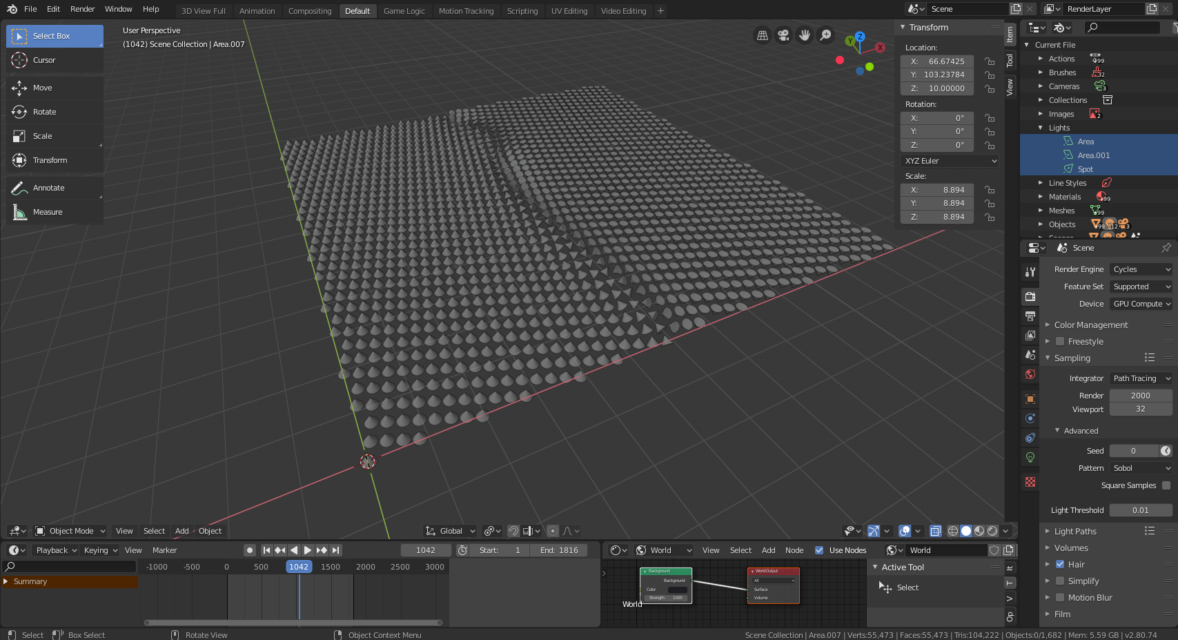
Here, colors is simply a list of RGBA tuples; for me, these were taken from the matplotlib RdBu_r colormap. After running this script, the Blender interface should look like this:

Now all that remains is to add lighting and cameras, and then render whatever animations or images we need.

Results

After spending more time than I'd like to admit keyframing camera motion and adding lighting, I was able to make an animation that I'm happy with. After rendering the animation using the fast Eevee render engine, I found that the animation was slower than I wanted it to be, but this was easily fixed by increasing the frame rate with FFMPEG. This animation shows how the domain wall propagates under the external magnetic field, and I think it captures its chaotic motion really well:

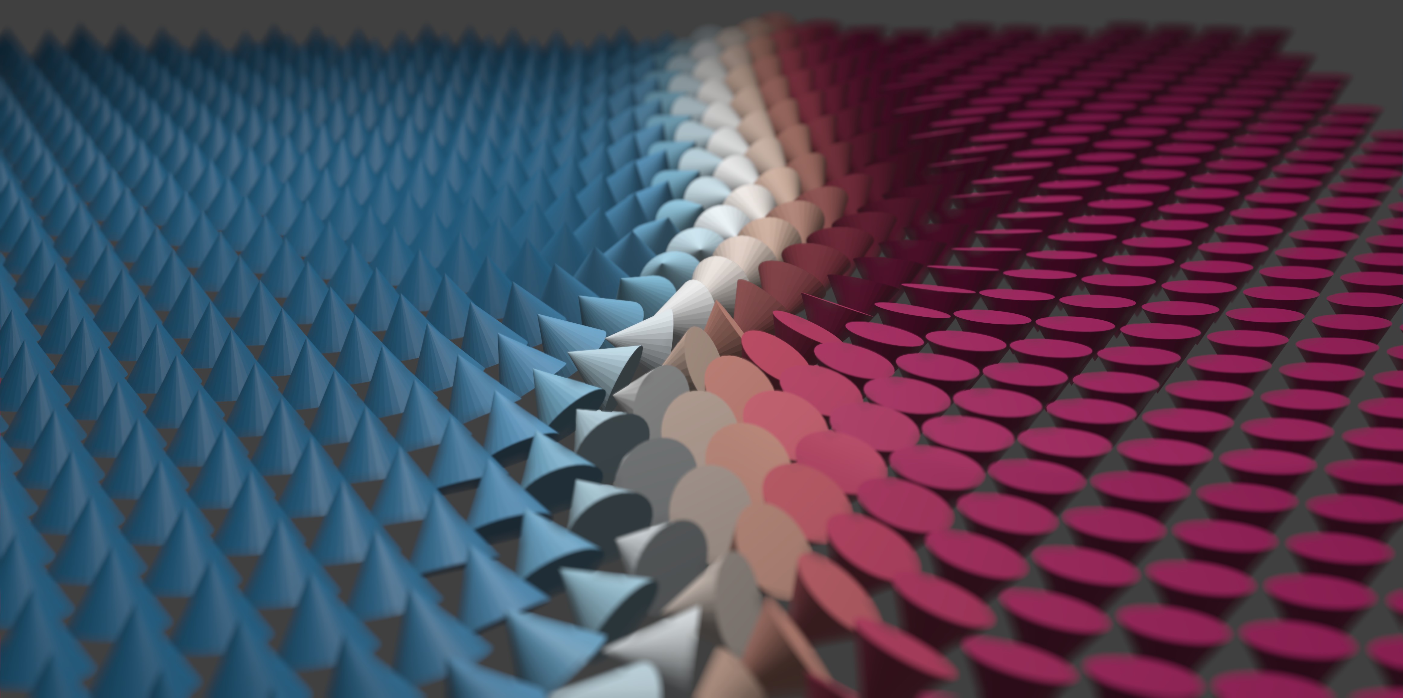
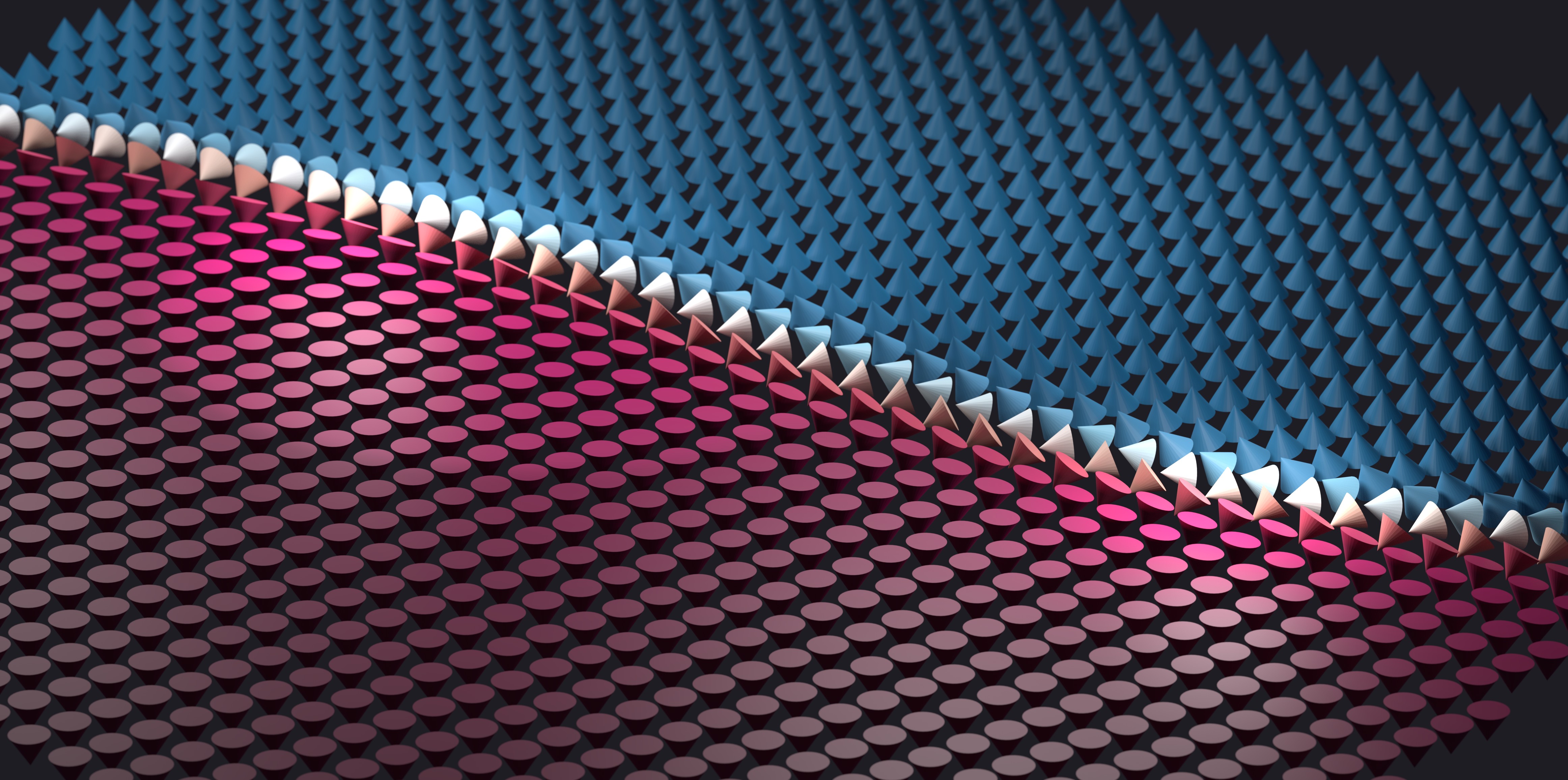
The z-component of the magnetization is used to color the cones: when the cone points up the color is red, and when it points down the color is blue. I also rendered a different pair of images of the domain wall which I used in a previous post as well:

The lighting and depth of field make these images so much more interesting! The time I spent learning to use Blender's Python API has really been worth it, and I think it will be useful for creating professional level data visualizations in the future. Bridging the gap from the Mumax micromagnetics simulator using a combination of custom Go functions and Python scripting took a significant investment of time and effort, but ultimately the payoff can be worth it.

Footnotes

1. While you can actually split this single mesh into a bunch of separate objects in Blender, this still doesn't really solve the problem. For example, suppose I have some object in Paraview which moves as a function of time, and I want to make a movie of it in Blender. I can try to export my data in Paraview as a set of PLY files (frame1.ply, frame2.ply, frame3.ply, ...), like frames from a movie. But there is still no way to tell Blender that the object I import from frame1.ply is the same object as in frame2.ply, shown at a different time. As far as Blender is concerned these are compeletely different objects, so Blender's most powerful animation features - specifically, keyframing the motion of objects - just won't work here. ↩

2. After posting this, I've discovered that you can in fact align objects to a vector using the mathutils.to_track_quat() function. Maybe I'll make another post about this later. ↩